In 2013, the Efficient Estimation of Word Representations in Vector Space paper was released introducing two new model architectures for generating vector representations (or embeddings) of words. While today more advanced models are in use, the Word2vec paper remains a popular classic that has been cited over 40,000 times.
In this post, we will implement the Continous Bag of Words (CBOW) model, one of the two architectures introduced in the paper. The goal of this post is to serve as a straightforward example of implementing a paper.
About Embeddings
Embeddings is a smart technique to encode and represent language. The problem with traditional one-hot encoding is that it doesn’t carry any sense of meaning about the captured words. The assignment from words to vector is arbitrary and relationships and similarities between words are not captured by the representation.
One-hot Encoding Problems
I want you to imagine with me the pain of building a model on a downstream task while representing words with one-hot encoding. Imagine that we are building a very simple binary classification model that takes as input a single word and predicts positive or negative sentiment (a trivial task). This model will pass the one-hot encoded vector to a single linear layer (note that the argument remains the same for deeper models). We will consider the deficiency of such representation in two aspects: quality and cost.
Quality
First I want to establish that this model will simply return for each word in the class which has the most number of occurrences in the downstream training data. Suppose that the vocab size is 5 and that a certain word \(w\) is represented by the vector \(v_w\). Suppose that the first index of \(v_w\) is 1 and the rest are 0.
\[
v_w = [1, 0, 0, 0, 0]
\]
After passing the vector to the linear layer, the output will be:
\[
o = w_1 * 1 + w_2 * 0 + w_3 * 0 + w_4 * 0 + w_5 * 0 + b = w_1 + b
\]
Where \(w_i\) is the weight of the \(i^{th}\) word in the vocabulary and \(b\) is the bias.
To generalize, give a vector \(v_w\) of size \(n\) where the \(i^{th}\) index is 1 and the rest are 0, the output of the linear layer will be:
\[
o = w_i + b
\]
So basically, the model is memorizing for each and every word it sees the expected output. No features, no understanding, no learning. It’s just an expensive lookup table.
Why is that bad? Downstream tasks tend to have much smaller datasets than the huge language datasets used to build word representations. Thus, many words will not be seen in the downstream task, and our table will just pick up a random class.
Consider this example which we will revisit later. Suppose that the downstream dataset contains the word “hunger” and successfully predicts it as negative. During inference, the model encounters the word “famine” which is not present in the training data. The model will have no idea what to do with it and will randomly pick a class. This is a problem because “famine” is very similar to “hunger” yet the model can’t realize that.
Cost
Continuing with the previous example, let’s assume that the vocabulary size is 1,000,000. The downstream model will have to learn 1,000,000 weights and 1 bias. The weights increase linearly with the vocabulary size. This is a disaster as vocabularies are huge. We will see later that a vector representation can do using less than 1% of the weights and still achieve better performance.
Vector Representation
The idea of vector representation is to project every word in the vocabulary to an \(n\)-dimensional vector space. This projection is done such that similar words are close to each other; hence, the location of the word and the values in the vector carry actual meaning about the word. This allows us to utilize large amounts of language data to understand the semantics of words and their relationships, simplifying any downstream task.
In the previous example, the model is no longer a lookup table but an actual model with generalization ability that can learn from the encoded information in the vector. Now, the model will be able to predict the class of “famine” because its vector is similar to that of “hunger” and hence will have a close output.
Summarizing the Paper
The first thing I want to highlight about the paper is its publishing date: 2013. Computation was expensive, models were small, and architectures were simple (no transformers yet). So as highlighted in the name, the goal of the paper is to establish an efficient technique to generate the vector representation.
At the time of publishing, the largest model made was trained on only a few hundred million words and had a dimensionality of 50-100. Using their proposed architectures, the authors succeeded in training on 6 billion words and a vector dimensionality of 300.
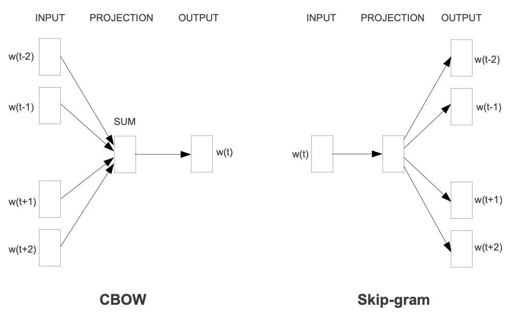
Two architectures are introduced: Continous Bag-of-Words (CBOW) and Continous Skip-gram. The CBOW model predicts a token by projecting the \(N\) preceding and the \(N\) succeeding token into their vector representation then summing them, normalizing the sum, and passing it to a classifier. In their implementation, they used a log-linear classifier with \(N=4\).
The Skip-Gram does the opposite by using a token to predict the neighboring ones. While training a number \(R\) is randomly selected from the range \(<1;C>\) where \(C\) is a hyperparameter. The \(R\) preceding and succeeding tokens of the current token are predicted from the current one.
To test the quality of the vectors, the authors create a comprehensive test set containing five types of semantic questions and nine types of syntactic questions. Each question is represented as two-word pairs. For example, a common capital city question would have word pair 1 \(<Athens, Greece>\) and word pair 2 \(<Oslo, Norway>\). In this case, the model will be tested by extracting the word whose vector is closest to
\[
vect(Athens) - vect(Greece) + vect(Norway)
\]
and assigning the prediction as correct if and only if the word is \(Oslo\).
This summary skips a lot of details which we will discuss only as needed in the implementation phase. We will implement the CBOW model.
Data Preparation
The dataset used in the paper is the Google News Corpus which contains 6 billion tokens. I have not been able to find a copy of the dataset so I will use the WikiText2 dataset by Salesforce which is much smaller allowing us to train the model quickly. We will use huggingface’s datasets library to load the dataset. Without further ado, let’s start coding.
The number above is the number of sentences in the train and test sets.
The first step is to define the method to tokenize the sentences. The paper did not mention any specific method so I will use the default sentence tokenizer from the nltk library on the lowercase version of the text. The tokenizer will split the text into words while maintaining punctuation.
Code
def tokenize(sentences):""" Tokenizes a list of sentences into words. Args: sentences (list of str): List of sentences to tokenize. Returns: list of list of str: List of tokenized sentences, where each sentence is a list of words. """return [word_tokenize(sentence.lower()) for sentence in sentences]
The next step is to create the vocabulary. To do so we will use the top \(N\) most frequent tokens where \(N\) is a hyperparameter. In the paper, the authors used a vocabulary size of 1,000,000 for a dataset of 6 billion tokens. We have a much smaller dataset so we will use a smaller vocabulary size of 10,000.
We add two important tokens: <pad> and <unk>. The first is used to pad the input sequences while the latter is used to represent unknown tokens, those out of the vocabulary.
Code
PADDING_TOKEN ="<pad>"UNK_TOKEN ="<unk>"VOCAB_SIZE =10000def build_vocab( corpus, vocab_size=VOCAB_SIZE, padding_token=PADDING_TOKEN, unk_token=UNK_TOKEN, tokenize_func=tokenize,):""" Builds a vocabulary from the given corpus with size vocab_size. Args: corpus (list of str): List of sentences to build the vocabulary from. vocab_size (int): Maximum size of the vocabulary. padding_token (str): Token used for padding. unk_token (str): Token used for unknown words. tokenize_func (callable): Function to tokenize sentences into words. Returns: A tuple containing: - vocab (list of str): List of most common vocab_size tokens. - token_to_id (dict): Mapping from tokens to unique IDs. - id_to_token (dict): Mapping from unique IDs to tokens. """ all_tokens = [ token for sentence_tokens in tokenize_func(corpus) for token in sentence_tokens ] token_counts = Counter(all_tokens) vocab = [token for token, _ in token_counts.most_common(vocab_size)] token_to_id = { token: idx +2for idx, token inenumerate(vocab)if token notin [padding_token, unk_token] } token_to_id[padding_token] =0 token_to_id[unk_token] =1 id_to_token = {idx: token for token, idx in token_to_id.items()}return vocab, token_to_id, id_to_tokenvocab, token_to_id, id_to_token = build_vocab(train_ds["text"])len(vocab), len(token_to_id), len(id_to_token)
(10000, 10002, 10002)
Note
Note that the length of token_to_id and id_to_token is greater than the vocabulary size by 2 because of the two special tokens.
The model can’t comprehend the text directly and we have to convert each word to a numeric id. We use the two dictionaries we created to convert the tokens to their corresponding IDs.
Due to the data, having very long sentences and very short sentences, even empty ones, we will filter out any sentence with less than 4 tokens or greater than 256 tokens. This is a hyperparameter that can be tuned later. The paper did not mention any specific method for filtering the sentences so I will use this method.
Combining all the steps above, we are now ready to create a function to preprocess lists of sentences.
Code
MIN_LENGTH =4MAX_LENGTH =256def preprocess( sentences, token_to_id=token_to_id, tokenize_func=tokenize, min_length=MIN_LENGTH, max_length=MAX_LENGTH, unknown_token=UNK_TOKEN,):""" Preprocesses a list of sentences by tokenizing and converting them to IDs. Args: sentences (list of str): List of sentences to preprocess. token_to_id (dict): Mapping from tokens to unique IDs. tokenize_func (callable): Function to tokenize sentences into words. min_length (int): Minimum length of sentences to keep. max_length (int): Maximum length of sentences to keep. unknown_token (str): Token used for unknown words. Returns: - tokenized_sentences (list of list of str): List of tokenized sentences. - sentences_ids (list of list of int): List of sentences represented as IDs. """ tokenized_sentences = tokenize_func(sentences) tokenized_sentences = [ tokensfor tokens in tokenized_sentencesiflen(tokens) >= min_length andlen(tokens) <= max_length ] sentences_ids = [ [token_to_id.get(token, token_to_id[unknown_token]) for token in tokens]for tokens in tokenized_sentences ]return tokenized_sentences, sentences_idstrain_tokens, train_ids = preprocess(train_ds["text"])test_tokens, test_ids = preprocess(test_ds["text"])
Now we have all the sentences in form comprehensible by the model. What we have to prepare now is the input and output for the model formatted in the way specified in the paper. For each token, we get the \(N\) preceding and \(N\) suceedsucceedinging tokens and call them the context and we call the token itself the target. The context is the input to the model and the target is the output. The paper used \(N=4\) so we will use the same value.
Code
CBOW_WINDOW_SIZE =4def create_cbow_data( token_ids, window_size=CBOW_WINDOW_SIZE, padding_token=PADDING_TOKEN):""" Creates CBOW data from token IDs. Args: token_ids (list of list of int): List of sentences represented as IDs with shape (batch_size, seq_len). seq_len can be variable. window_size (int): Size of the context window. padding_token (str): Token used for padding. Returns: A tensor dataset containing context and target pairs. Context Shape: (L, 2 * window_size). Target Shape: (L,) where L is the sum of the lengths of all sentences in token_ids. """ contexts = [] targets = []for tokens in token_ids:for i, target inenumerate(tokens): start = i - window_size end = i + window_size context = [ tokens[j] if j >=0and j <len(tokens) else token_to_id[padding_token]for j inrange(start, end +1)if j != i ] contexts.append(context) targets.append(target)return TensorDataset( torch.tensor(contexts, dtype=torch.long), torch.tensor(targets, dtype=torch.long), )cbow_train = create_cbow_data(train_ids)cbow_test = create_cbow_data(test_ids)
Model Definition
We now extend PyTorch’s nn.Module class to create our model. This model will implement the CBOW architecture but I will use a linear layer instead of a log-linear classifier for simplicity. Another change is that all embeddings will have a max l2 norm of 1 to prevent the vectors from exploding. In the paper, the sum of the embeddings was the one normalized.
We also define a method called get_embeddings which will return the embedding of a token given its ID.
Code
class CBOW(nn.Module):""" Continuous Bag of Words (CBOW) model for word embeddings. Args: vocab_size (int): Size of the vocabulary. embedding_dim (int): Dimension of the word embeddings. padding_idx (int): Index for the padding token. normalize_embeddings (bool): Whether to normalize the embeddings. """def__init__(self, vocab_size, embedding_dim, padding_idx=0, normalize_embeddings=True, ):super(CBOW, self).__init__() max_norm =1.0if normalize_embeddings elseNoneself.embeddings = nn.Embedding( vocab_size, embedding_dim, padding_idx=padding_idx, max_norm=max_norm )self.linear = nn.Linear(embedding_dim, vocab_size)def forward(self, context): embeddings =self.embeddings(context) embeddings = torch.sum(embeddings, dim=1) output =self.linear(embeddings) log_probs = torch.log_softmax(output, dim=1)return log_probsdef get_embeddings(self, token):returnself.embeddings(token)cbow_model = CBOW( vocab_size=len(token_to_id), embedding_dim=300, padding_idx=token_to_id[PADDING_TOKEN],)
Training the Model
We first define the dataloaders. I will use a batch size of 256. You can change that based on your GPU memory.
We will now create the training loop. Following the paper, we will use AdaGrad as the optimizer and use a linear learning rate scheduler starting from 0.025 and decaying to 0 in the end. We will also use 3 epochs to train the model.
Epoch 1/3: 0.4458 in top 10
Epoch 2/3: 0.4424 in top 10
Epoch 3/3: 0.4413 in top 10
Conclusion
In this post, we implemented the CBOW model, a classic model introduced in the Word2Vec paper. The goal of this post was to show a simple example of implementing a paper. I hope you found this post helpful and helped you understand more about NLP.